It is recommended to read the FAQ first before searching here for answers.

The full copyrights of this documentation, including the figures, remain to the author. Please contact spisop@spisop.org if you want to use any of the figures or text here.

Disclaimer & Licensing: This Documentation does not claim completeness of correctness of all the procedures mentioned. However the author tried to convey as much as possible. The Backgound section below does not accurately reflect the current scientific state of the art. It reflects the authors opinion on what he thinks is useful to consider to run and understand the rationaly behind common analyses procedures. Most of the content refers to human EEG and would differ for animal recordings. Any comments and suggestions or hints that are helpful to improve this documentation are highly welcome and can also be adressed to spisop@spisop.org 

The SpiSOP software is free; you can redistribute it and/or modify it under the terms of the GNU General Public License as published by the Free Software Foundation; either version 2 of the License, or (at your option) any later version (e.g. version 3).

This program is distributed in the hope that it will be useful, but WITHOUT ANY WARRANTY; without even the implied warranty of MERCHANTABILITY or FITNESS FOR A PARTICULAR PURPOSE. See the GNU General Public License for more details. THIS SOFTWARE IS NOT INTENDED FOR CLINICAL DIAGNOSES AND SHOULD NOT BE USED IF LIFES ARE AT STAKE.

You should receive a copy of the GNU General Public License along with the software; if not, write to the Free Software Foundation, Inc., 59 Temple Place – Suite 330, Boston, MA 02111-1307, USA.

Background

Sleep stages and scoring

There is Wake, MT (Movement Time), Stage 1 (S1), Stage 2 (S2), Stage 3 (S3), Stage 4 (S4), REM (Rapid Eye Movement), where SWS (slow wave sleep) = S3 + S4 and NonREM = SWS + S2 (please note, event though S1 is a NonREM stage this it is not considered here as such for the use in the toolbox for the lack of characteristic sleep events). This is an extention of the sleep scoring suggested by Rechtschaffen and Kales 1968. It is “compatible” with the AASM scoring rules when using N1 = S1, N2 = S2, N3 = S3+S4, REM = REM and NonREM = N2+N3.

Sleep onset time refers to the onset of the first S1 epoch after lights-off that is followed directly by only S1 and NonREM (but not wake) epochs.

S2 onset, SWS onset and REM onset refer to the onset time of the first respective epoch since sleep onset time.

Total sleep time (TST) is the time from sleep onset to first wake epoch not followed by a sleep epoch (i. e. S1 or NonREM, usually after lights-on markers, however lights-on markers are not considered in SpiSOP).

Sleep stages can be scored with the software “Schlafaus” (by Steffen Gais) or the SpiSOP browser, as they are needed as input for SpiSOP. See Figure 1 for illustration of the above.

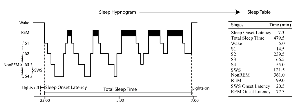
Figure 1: Example sleep hypnogram over a full night demonstrating how sleep scoring parameters like Sleep Onset Latency are calculated and transformed into a sleep table according to Rechtschaffen and Kales 1968. Note that this example does not show small Wake periods after sleep onset, typical for a real hypnogram.

 

Sleep spindles

Sleep spindles can be classified in two types, slow (~9-12 Hz) and fast (~12-15 Hz) spindles, both occurring mostly during NonREM sleep with a duration of 0.5 to 3 s (or 0.3 to 3 s, or 0.5 to 2 s, usually little bit less than 1 s on average) and with a waxing and waning of the peak or trough amplitudes. Maximal peaks and troughs can mark the center of a spindle (usually the trough is preferable).

The exact frequency of each spindle type varies (greatly) between individuals, (moderatley) nights and  (moderately) sleep stages.

Therefore these individual frequencies have to be determined in the frequency power spectra between 8 and 18 Hz as the peaks in NonREM sleep stages (e.g. with function freqpeaks). In adults slow spindles (< 12 Hz but above 9 Hz, usually not higher than 11.5 Hz and on average 10.5 Hz) show higher frequency power in frontal channels mostly during SWS and temporally often coocurring before or after fast spindles (12-14 Hz and ~13.3 Hz on average), which show higher power in parieto-central channels and are present throughout whole NonREM with comparable density (although not directly visible during SWS). Slow spindles are thus easier to find in frontal-channesl over SWS epochs and fast spindles in S2 sleep or all NonREM in centro-parietal channel (recommended procedure).

Some researchers also define slow and fast spindles differently, as the slow and fast components of fast spindles (<13 Hz slow, and > 13 Hz as fast). This split of fast spindles gives further complications and considerations since this eventually splits spindle events by half for some subjects more than for others.

Often no clear slow (or fast) peak of the spindle frequency in the power spectra can be found in NonREM sleep stages and imputation has to be performed on several data sets (e.g. replace later by group mean frequency or take the one where the power is at least not too low). See Figure 2.

One might consider concentrating on the respective sleep stages and channels to find the peak frequencies of the respective spindle type.

Spindle events should be temporally aligned to either their maximal trough (minimum trough potential) or maximal peak.

Slow oscillations

Slow oscillations occur mostly during NonREM sleep. They can be classified in high amplitude slow oscillations (0.5-1 Hz, ~0.8 Hz in humans) and lower amplitude delta waves (1- 4 Hz), both of which show amplitudes of at least 75 µV in scalp EEG sleep recordings. In adults they mostly originate from frontal areas and seem to “travel” to centro-parietal areas.

The core frequency of these slow oscillations refers to the duration of down and up peak. On average a relatively fast and steep down peak is precedes by a longer and lower amplitude up peak. This irregularity therefore needs a prefiltering of the data that allows the frequency component of the down peak still to be included (e. g. prefiltering for 0.5–1 Hz slow oscillations is therefore low pass filter around 3.5 Hz).

One should use the negative half-waves lowest down-peak in the potential for the temporal identification of slow oscillations time-points because they typically show more discrete peaks in the EEG compared to positive half-waves, which have a broader and more variable shape (but can also be used depending on the question to be answered).

 

Power-spectral-density and Power Spectrum band estimates

For analysis of the power spectral density (PSD) or the power spectrum (PS) in specific frequency band, several steps are performed:

Segmentation: The epoched data is further cut into time segments (aka. windows) of a specific length (e.g. 5 s) that either overlap (0.9 overlap) or do not (0 overlap). Depending on the segment length and overlap, some data is lost due to this segmentation. At most this is:

loss = (segment length * (1 – overlap)) * (number of consecutive epochs of sleep stages of interest)

e.g. if you have 10 NonREM consecutive data parts due to epoching, 5 s segments and 0.9 overlap, then the segments will not cover at most (5 s * (1 – 0.9)) * 10 = 5 s. Note that this “maximal lost coverage” is at the end of those consecutive data parts, each of maximal length (segment length * (1 – overlap)). The segment length should not exceed the epoch length (humans usually 30 s and rodents 10 s or 4 s). This means for usual human scorings the maximal segment length should be chosen to be 30. (A future release will also be able to handle less loss and thus smaller segments, due to adaptation of the window function, see further below)

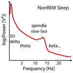
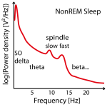
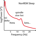
Figure 2: Example of three power spectra from NonREM Sleep EEG data (e.g. around Cz). Not in all individuals there are two clear power peaks (left power spectrum) and often the slow spindle power peak (left power spectrum) is missing (center power spectrum) or hidden (left power spectrum) .

 

Accuracy/spectral resolution sonsiderations: The maximal frequency resolution that can be used is f_res = 1/(segment length in seconds) = f_s/N, where f_s is the sample frequency of your data (e.g. 500 Hz) and N is the segment size/length in samples. Always compute f_res before you even think to start power spectrum estimation.! For example for 5 s segments the frequency resolution is 1/(5 s) = 0.2 Hz thus the spectrum will result in those frequency bins/steps by 0.2, 0.4, 0.6, …

Hint: You do not have to consider if the segement length is of specific sample length satifying the power of 2 law for very fast fourier transform (e.g. 128, 256, 512 … samples). The fast fourier transform performed here is also very fast for any length of samples, and as accurate too, so you have the power to choose.

Calculation: The Power Spectrum is estimated by calculating a transformation of the signal in each segment using fast fourier transformation (FFT), but only after the segments have been “tapered”. In the simple case this tapering involves using a single taper (here a single Hanning taper is used), i.e. limiting the signal of each segment by a so called “window function” (Figure 3.1 and Figure 3.2). For example, lets take the Hanning window function, that attenuates the signal at the beginning and end of segments. Note that for the Hanning window an overlap of 0.5 is sufficient, however if you want to avoid mentioned data loss due to segmentation procedure and still keep a sufficient frequency resolution using large Segments (f_res) you need to use a higher overlap of 0.9. Overlap values between 0 to 0.5 and 0.5 to 0.9 should not be chosen. High segment overlap can also lead to redundant calculation of the same signal, and of cause an increase in computation time.

The purpose to use such a spectral window function and limit the signal for each segment is to reduce “leakage” aberrations in the following FFT output. Such leakage appears because sudden changes in the data at the start and end of each segments. Therefore the window reduces the amplitude (and therefore the power) of the signal in the segment especially at the ends. The trade-off for this tapering method is that the frequency resolution is also reduced, and is attributed to a simple lack of data points for each FFT calculation. NEW, the window function can also be modified by adjusting the proportion of the hanning window (only works with hanning window) that is applied. e.g. 1 means 100% of hanning window applied and 0.5 means 50% of hanning window with symmetrically 25% of each segment tail (left and right) given a hanning shape (Figure 3.1)

 

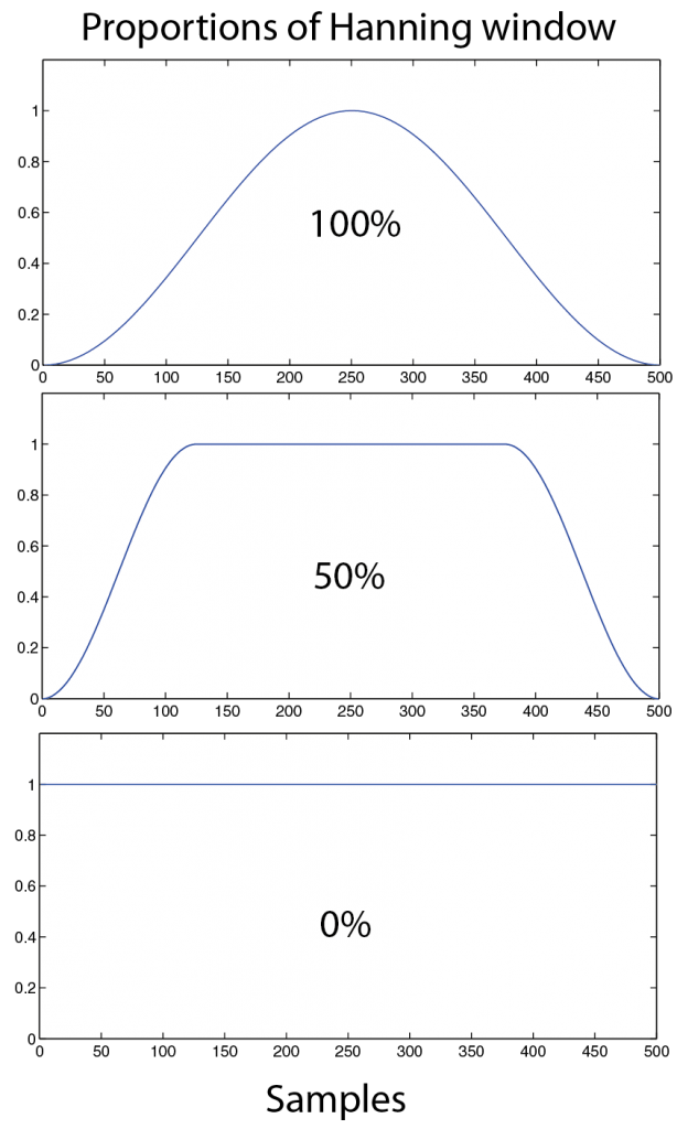
Figure 3.1: Example of how a window function (here a Hanning window in blue) is adjusted by a proportion (in %) and how this influences the shape, 100% is the usual standard hanning window. 50 % is stable and uses more of the tails. 0% is square shaped and does interfere with the following FFT calculation.

Therefore spectral windowing of each segment improves accuracy of the power spectrum estimation, however the contribution to this estimate of the signal would be reduced near the beginning and end of the segments. This is why we overlapped the segments in the first place. This overlapping compensates – at least to some degree – for the lower contributions at the boundaries of the hanning-tapered segments. The resulting power estimates for each overlapped segment is then averaged across all segments (Welch’s overlapped segmented average). See Figure 4. Averaging therefore reflects the average power spectrum of the whole data of interest (or all data parts), i.e. one frequency relative to the other frequency in all the data. However one can also get another arbitrary estimate reflecting an absolute measure of power of a frequency by adding (instead of averaging) across all power spectra. This “summed” power reflects therefore a quantitative measure of total power observed across the data of interest. For example if you are more interested in frequency increases relative to the other frequencies within one data set use the averaged values. If you are rather interested in the “amount” of frequency power observed in each dataset, then use the summed power spectra. Consider that both, summed and averaged, power spectra values can also be normalized by dividing and multiplying by the length of the data of interest (data region of interest, aka. data ROI), respectively.

Average over Bands: Well if we now have the power spectra as we want it (averaged or summed), we can “cut out” the values of some interesting frequency bands (with a specific cutting accuracy that should not to be conflicted with f_res). See lower part of Figure 4. For example we want to cut from 4 Hz to 8 Hz. Consider that frequency resolution is for example f_res = 0.2 Hz). This results in ((8-4)/f_res) + 1 =  (4/0.2) + 1= 21 power values. Those 21 power values reflect then the theta band and are averaged to one value, that then is a representative for this theta band. This can be done for all other frequency bands within a minimum frequency of f_res and a maximum frequency of half the sample frequency i.e. f_s/2 (aka. the Nyquist frequency), e.g. if the sample frequency f_s is 500 and segment length is 5 s then the minimum frequency is 0.2 Hz and maximum is 500/2 = 250 Hz.

Common used frequency bands of sleep EEG (often exact frequencies vary between labs, studies and species, here for humans):

slow oscillation (SO) 0.5 – 1 Hz

delta waves 1 – 4 Hz

slow wave activity (SWA) 0.5 – 4 Hz

theta 4–8 Hz

(alpha 8-12 Hz, overlapping and confounding for the “slow spindle band”)

slow spindle 9–12 Hz

fast spindle 12–15 Hz (also called sigma)

beta 16–30 Hz

slow gamma 30–45 Hz 

fast gamma 60–90 Hz

 

NOTE: Please consider not to rely on signals from the 50 Hz (e.g. Europe) or 60 Hz range (e.g. US), since this reflects the power line hum prevalent in most recordings (if no specifically taken care of at recording). SpiSOP by default filters 50 Hz and multiples (100 Hz, 150 Hz) (and can be changed in the Core parameters to 60 Hz) noise out, however this is never perfect!

 

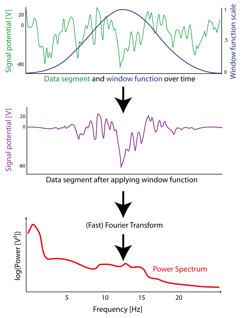
Figure 3.2: Example of how a window function (here a Hanning window in blue) is applied (sample-wise multiplication) to signal (green) of a segment of data resulting in an signal that is attenuated at the borders (purple). After “windowing”(or ”tapering”) of the windowed signal a Fast Fourier Transform (FFT) can be applied to estimate the power spectrum (red) of this particular segment.

 

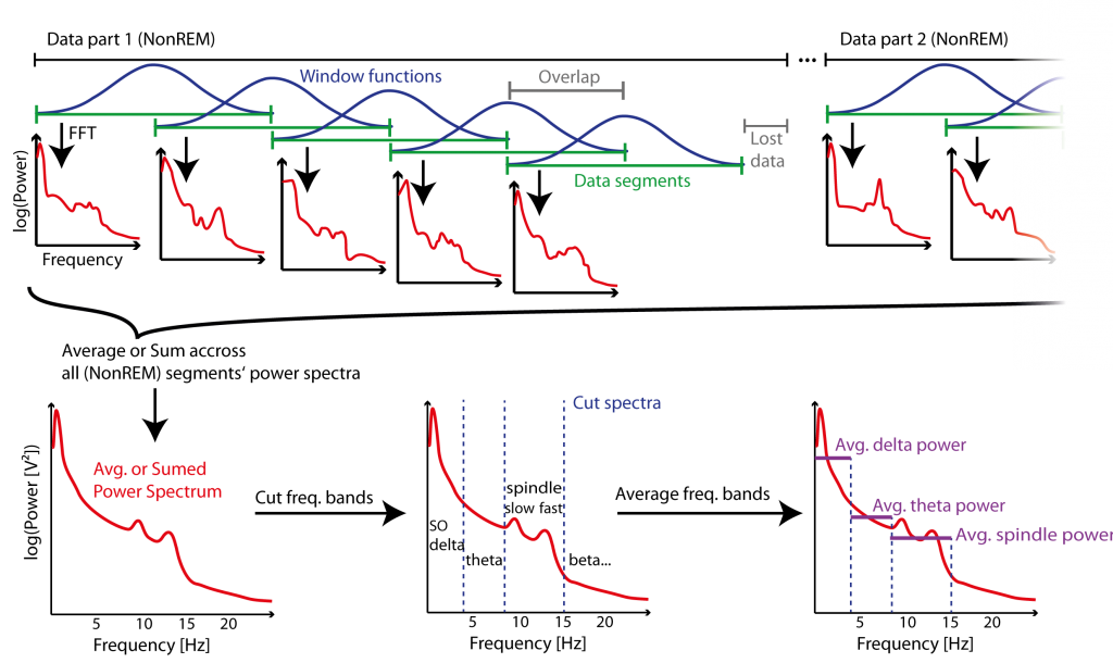
Figure 4: Example of Segmentation method (Welch’s Method) for Power spectrum estimation of several parts of data. Data is segmented in segments (green) of a fixed length, and a window function (blue) is applied to the signal of those segments to prevent “spectral leakage” for the then applied fast Fourier transformation (FFT) that estimates the power spectrum (red) of each segment. Segments overlap to compensate for the loss of power at the boundaries of each segment – which is a result of windowing – and also to reduce lost data (grey) at the end of consecutive data parts. Power spectrums across segments of all data parts are then averaged (or summed to give a energy measure) to give a power spectrum estimate representing the whole data. The specific frequency bands are cut from the power spectrum and then averaged within those bands (purple) to give power estimates representative for those bands.

Note that calculating the power spectra for lower frequencies takes more computation time (“the lower, the longer”).

Power Density: However, for now the calculation only resulted in power estimates for each frequency, i.e. a power spectrum (PS) estimate. How do we get an equivalent power density (PD) estimate for each respective frequency, i.e. the Power-spectral-density (PSD) estimates? And what is the difference between power and power density? Simply speaking, the difference is that PSD does not depend on the parameters you used for the FFT on the segment signals, i.e. varying segment size and the applied window function. Therefore we need to normalize the power estimates to obtain power density estimates. We do this using the Effective Noise BandWidth (ENBW) calculated by a window function specific constant Normalized Equivalent Noise BandWidth (NENBW) and the frequency resolution f_res (aka. frequency bin size for the FFT). Let’s assume we used EEG and our measured signal potential is Volts [V]. Since we normalize the power (for the whole spectrum) [V²] by a frequency (i.e. a band width), the power density (for each value in the spectrum) unit is now [V²/Hz]. For further details, e.g. how to calculate NENBW from any discrete window function and sample frequency and also why the following calculations are valid see Heinzel et al. 2002 (pdf can be found in the literature folder (if supplied) or online GH_FFT.pdf a good introduction from G. Heinzel , A. Rudiger and R. Schilling).

The calculation is relatively simple once the already mentioned values are known:

PSD = PS / ENBW

or power density = power / ENBW

, where

ENBW = NENBW * f_res = NENBW * f_s / N = NENBW / (segment length)

, and where f_s is the sampling frequency

, and f_res the width of one frequency bin (e.g. 0.2 Hz)

, and N is the segment size/length in samples N = (segment length) *f_s.

NENBW remains constant for single taper windows.

For the Hanning window we have  NENBW = 1.5 bins.

(For the Hamming window we have NENBW = 1.3628 bins.)

Note that PSD estimates for multi-taper methods (usefull for shorter data segments not typical for sleep EEG) is not supported by SpiSOP yet, but maybe in a future release.

On the output:

Name	Relation	Unit (with Volt as Potential)
Power spectral density (PSD)	PSD = PS / ENBW	V²/ Hz
Power spectrum (PS)	PS = PSD * ENBW	V²
Linear (/amplitude) spectral density (LSD) or “Energy spectral density”	LSD = sqrt(PSD)	V
Linear (/amplitude) spectrum (LS) or “Energy spectrum”	LS = sqrt(PS)	V/sqrt(Hz)

 

Consider also other potentials than Volts [V] for EEG and MEG and their cardinalities, e.g.  [µV], [mV] and Tesla [T] [fT/cm²].

 

Note, the Nyquist-Shannon sampling theorem still should hold (http://en.wikipedia.org/wiki/Nyquist%E2%80%93Shannon_sampling_theorem), i.e. the sampling frequency of the data f_s must be higher than the maximal frequency of interest. For example if your sampling frequency is 200 Hz then the maximal frequency you can include use is therefore < 100 Hz, i.e. for example 100 Hz minus f_res (e.g. 99.8 Hz). However in practice, use less than approximate 90 Hz since 90 * 2.2 < 200 Hz, SpiSOP requires a three times higher sampling frequency thant the to be inspected frequency (so up to 66.6 Hz inspected frequency for a 200 Hz signal frequency)

 

Methods and Algorithms implemented in SpiSOP

Important general remarks

Filtering or prefiltering is always performed on the original sample frequency before putative down sampling of the data for further analysis.

Data is used only from the given sleep stages of interest excluding epochs manually scored as movement arousals or artifacts.

This results in consecutive data blocks of interest with a minimum length of one epoch length (e.g. 30 s).

Only dataset specific channels of interest are used for analysis. Channels can be averaged before analysis as one virtual channel.

For each event also the sleep stages – according three “scoring levels” –  is given.

For each run of an analysis function a smaller subsets of datasets can be chosen.

The first scored epoch in the hypnogram (scoring files) is assumed to contain the first sample of the dataset. Scoring of Analysis relevant sleep stages should not be longer than the actual data, in this case a warning is given that the further scored part is not incorporated in the analysis.

If set parameters do not match the data (for example sample frequency) then errors are reported and suggest what to change or adapt in order to re-run the analysis.

Always perform a prefiltering of your datasets when they were recorded without filtering. You can use the preprocout function to do this, but every SpiSOP function conservatively filters the data again, just to make sure it is fit for the necessary analysis steps. Important one cannot get frequency information beyond this (pre)filtering. Also if for example the data has been already low-cut filtered for 0.159 Hz and high pass filtered for 35 Hz, one can only look in this (band-pass) range of 0.159–35 Hz. Filter settings could be obtained from looking into the header files , e.g. fro brainvision files note that a time constant of 3 s results in 1/(2*pi*3 s) = 0.054 Hz low cut-off frequency, if time constant is 1 s then this corresponds to approx. 0.159 Hz. Note that if data is already pre-filtered (especially for low frequencies) no further pre-filtering in the parameters of the analysis function might be set, i.e. set high pass filters to 0 Hz which results in no high pass filtering at all (since data was already filtered)!

 

Hypnogram values

Sleep values for creating a sleep table are created from the hypnograms (files) obtained from sleep scoring and from a list of lights-off periods (given in non-negative samples offset from start of data) for each dataset. This includes the total sleep time (TST) and the amount of each sleep stage or level of sleep stage in percent (of TST) or absolute duration (in minutes). Separately the same percentages and duration are obtained for artifact (no movement arousal) epochs. Additionally general sleep onset (after lights off), and onset times of important sleep stages (after sleep onset) are given too. Sleep onset is referenced to given Lights-off time-points (in samples after start of EEG recording, or giving an additional offset) for each dataset separately (see FAQ on the data format requried)

 

Filters

There are four filter types supported: (1) FIRdesigned (2) IIRdesigned (3) fir (4) but .Filter (1) and (2) are the default Finite Impulse Response (FIR) equiripple and infinite Impulse Response (IIR) Butterworth filter, respectively. Filters (3) and (4) are the FIR (hamming window based) and IIR (also butterworth) filters used by the fieldtrip toolbox, respectively. Filter parameters and designs for band pass, high pass and low pass filtering can be changed, default values are two-pass filters (matlab zero-phase filtfilt two-pass filter function), however also one-pass filters can be chosen. Note that in case of two-pass of a filter that filter attenuates the signal twice as much as in one-pass and therefore changes the given or reported cut-off frequencies accordingly. This two-pass double attenuation can be compensated automatically for FIRdesigned filters by dividing attenuation values by two. All high pass filters are by default IIR Butterworth filter of 4^th order with cut-off frequencies given in -3 dB (parameter: IIRdesigned as default or but for fieldtrip version). Low and band pass filters are FIR equiripple (default) or FIR Hamming window (parameter: IIRdesigned for equiripple as default or fir for hamming window based from fieldtrip) filters with a default attenuation of 100 dB in the stop band and 0.001 dB in the pass band. Transition width form pass to stop frequencies for FIR equiripple filter can be modified but are at 1.25 Hz transition width by default. Alternatively for Attenuation values a fixed filter order can be specified. Note that is case of the fieldtrip implemented filters the frequencies given are NOT pass frequencies but cut-off frequencies with -6 dB cutoff for FIR Hamming window (parameter: fir) and -3dB cutoff for the Butterworth filter (parameter: but). Clear filter properties can only be reported for parameters FIRdesigned AND IIRdesigned, otherwise they have to be approximated using a filter designed outside the toolbox, in this case (using fir or but) also the fixed filter orders should be stated in the parameters for each filter type. In case of fir the default filter order is 3*floor(f_sample / min(f_cutoff)), e.g. for 100 Hz sampling rate of a band filter between 10 and 15 Hz is 3*floor(100/min(10,15) = 3*floor(100/10) = 3*10 = 30, however more than 500 is recommended to obtain accurate attenuation.The filter order should not exceed floor(f_sample * (epoch length)). All functions implement an additional high pass filter that can be applied previous to downsampling. Note if this pre-downsample high pass filter is not turned off, it will filter also in the case that no downsampling is required (for compatibility reasons with other datasets that might need downsampling). In case data is already pre-filtered (during recording for example) the pre-filter can be turned off (set to 0 Hz filter).

Before downsampling (and after pre-downsampling high pass filtering) from frequency f_ori to f_down, a standard low pass FIR (Kaiser window, beta = 5) filter is applied to reduce aliasing effects (this filter is the standard resample filter of the FieldTrip toolbox and is realiesed with the firls matlab function). Unlike the other filters this filter cannot be modified in any parameters. If the ratio f_down/f_ori = p/q then the filter order is N = 2*10*q, e.g. downsampling form 200  Hz (f_ori) to 100 Hz (f_down) results in a filter order of N = 2*10*2 = 40, since 100/200 = 1/2 = p/q.

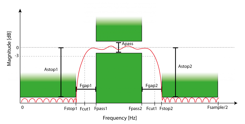
Figure 5: Example of FIR equiripple band pass filter characteristics. Magnitude of filtering depends on frequency and filter order, defined by minimal attenuation in the stop bands (Astop1, Astop2, defined by Fstop1 and Fstop2) and attenuation fluctuation in the pass band (Apass, within Fpass1 and Fpass2). The filter has a roll-off with transition to the stop bands with a gap (Fgap1, Fgap2) and defined by the -3db cut-off frequencies (Fcut1, Fcut2).

Power-spectral-density and Power Spectrum band estimates

Power spectra are determined by calculating the Fast Fourier Transformations (FFTs) to consecutive overlapping segments of a specific length (e.g. 10 s) and a specific overlap (e.g. 0.5), whose signal is limited by a Hanning window (single hanning-taper) resulting in a power spectum of the frequency resolution of 1/(segment length) Hz. Similarly a multi-taper DPSS (discrete prolate spheroidal sequence) or Slepian window approach instead of the single hanning window can be used with a specified smoothing frequency parameter (e.g. 0.1 Hz). The resulting power spectra across all segments are then averaged or summed. From the power values of each frequency then corresponding and power density values are calculated, i.e. for the hanning-taper approach, normalizing the spectrum for the segment size and the hanning-window applied. For further details see the same subsection under the Background section. For given frequency bands of interest the mean power (or power density) values are calculated form the averaged or summed power spectra (or power density spectra). Reported are the power and power density estimates for each band in each channel of interest (band_channel file) and the full spectrum, given in the maximal frequency resolution for each channel (full_channel file). Files for each individual dataset are then merged to a single file containing all entries of all analyzed datasets. It is checked if pre-filtering or data sample frequency or down sample frequency matches the requirements to obtain correct power spectra for the requested frequency bands. Bands are listed in an input file that can be adapted for band definitions. Full spectra are obtained from the range of minimal to the maximal frequency across all listed bands.

 

Frequency peaks for spindles or slow oscillation center frequencies

Computation of the power spectra is like methods in power spectrum bands estimates, however only in one spectrum of interest that is given by a minimum and maximum frequency. Note that the frequency resolution of the spectra depend on segment length f_res = 1/(segment length). Either detection of one peak or two peaks with a specific distance (e.g. 1 Hz) in the spectrum are (tried to be) automatically detected, however have to be visually accepted or adapted after computation by the experienced user. Visual confirmation and adaptation of each spectra of a dataset is done in a pop up window after all spectra are computed. Power spectral for visual inspection is smoothed using locally weighted scatterplot smoothing (LOWESS) with a 1 Hz frequency window.

 

Spindle detection

Spindle detection is based on (Mölle et al. 2002), but also see (Ngo et al. 2013). The algorithms were further adapted to get more properties and flexibility and include other approaches for finding spindles as is described in the following.

For the detection, one has to determine the center frequencies of spindles (either fast or slow) for each dataset or individual.

Then each EEG channel of interest in each dataset is band pass filtered using a finite impulse response (FIR) filter. The filter band is defined according to the dataset specific center frequency plus minus a frequency bandwidth constant for all datasets (band pass frequencies). The resulting frequency band can be further limited by general minimal and maximal frequencies across all datasets. For example previous determination of fast spindles center frequency in one dataset was 13.3 Hz, with a plus of 2 Hz and a minus of 1 Hz this gives the filter band of 12.3 to 16.3 Hz that can be further limited by minimal frequency of 12 Hz and a maximum frequency of 16 Hz and results in a frequency band of 12.3 to 16.0 Hz.

Then the root mean square (RMS) of the signal in a specific time window (e,g. 0.2 s) is determined for each sample resulting in a moving RMS signal. The moving RMS signal is further smoothed by a moving average of another window length (e.g. again 0.2 s). The samples of half this (maximal) window sizes, or the samples corresponding to sample frequency per minimal filter frequency (depending on what has more samples) are ignored at the borders of consecutive data blocks (data parts determined by hypnogram). The smoothed moving RMS signal is then used to detect spindles. The beginning and end of a putative spindle is marked, if the smoothed moving RMS exceeds a specific threshold for the length of an event-limiting time window that marks the minimum and maximum duration of the spindle event (e.g. 0.5 to 3 s). See Figure 6.1.

The threshold is expressed as a factor in units of (a) standard deviations (e.g. 1.5 SD) (b) mean of the positive signal half (e.g. 4 means),

of the (1) filtered signal or (2) envelope of the filtered signal,

either in the (x) respective channel, (y) the mean standard deviation of all channels of interest or (z) the standard deviation of all values across channels of interest. (,i.e. 2x2x3 = 12 parameter combinations)

Furthermore, since the moving RMS does not represent the envelope well, also the option is given to use the absolute values of the hilbert transfrom of the filtered signal, giving a precise envelope.

Also the option of a second threshold is given the envelope must surpass (at least once) in addition (criterion) to being counted as spindle. This accounts more for the waxing and wanning of the spindle, while better defining the beginning and the end of it. An illustration of using hilbert envelope and two thresholds is given in Figure 6.2.

For the putative spindle in the signal the following properties are determined from the filtered signal:

• Length (or duration) of spindle is the end minus the beginning time-points, both determined by the (lower) threshold crossings,
• peaks and troughs (trough = down peak) are the positive and negative extrema in the filtered potential, respectively. Within troughs or within peaks, respectively,  at least a minimum duration of a half wave of the max frequency of interest is reqired.
• The count of peaks and the count of troughs is given by the respective number of found extrema.
• Maximum peak and maximum through (minimum potential, that is negative in filtered signal) are the most extreme values of all troughs or peaks, respectively.
• Maximum trough to peak potential is the absolute potential difference between the maximum through and peak of a putative spindle.
• The average frequency of a spindle is determined by the mean of peaks and throughs count divided by the length of the spindle, i.e. (#peaks + #troughs)/(2 * length of spindle).
• Samples and/or time-points of the begins, ends, peaks, troughs, maximum peaks, maximum troughs are reported. Also the standard deviation within the filtered signal of the spindle is given to exclude further outliers after detection is finished. Reporting also includes other options.

Putative spindles can be merged before determining their properties if their boundaries (begins and ends) are in a proximity of a specified duration (e.g. 0.5 s). To assure merging is NOT applied in a sequential manner (i.e. no bias for merging of slow spindles that closely follow faster ones) this is performed in a greedy strategy:

The putative spindles are ordered in an ascending manner with respect to their boundaries difference. In one run, beginning with the putative spindles with the least boundary difference, two spindles are merged if they still confer with the limiting time window. If two merged spindle were merged in one run, then they are excluded from being merged again with other putative spindles until all further boundary differences are processed to be merged or not. This results in the first run, where two putative spindles were merged first, if their time difference of boundaries was also first, and second, if their boundary difference was second etc. The new set of resulting putative spindles is then ordered again and merged in the same manner in further runs. This continues until in one run no spindle can be merged again with any other spindle within the limits of the time window.

The merging count of how many putative spindles contributed to the final spindle set and to each resulting spindle are also reported.

Spindles can be further excluded if they do not concur with a maximum or minimum trough to peak potential, given in absolute values of the potential (e.g. 200 µV).

The final spindles are ordered to their time of occurrence also given a specific identification index within each channel that reflects the temporal ordering.

Report of spindles events includes each event and its properties (event file), an aggregation by channels of interest with key mean or summary values (channel file), and also each of the troughs and peaks of each spindle (two files with events, where each line corresponds to the respective line in the event file). Files for each individual dataset are then merged to a single file containing all entries of all analyzed datasets.

 

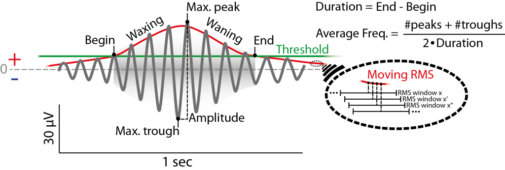Figure 6.1: Example of (fast) spindle in the filtered signal (12-15 Hz) and its definition by the detection method used. Detection is based on a threshold (green) passing of the root mean square of a moving window (red, magnification on the right) of the filtered signal. Threshold can be absolute Potential value, but usually is a multiple (e.g. 1.5) of the standard deviation of the whole filtered signal (e.g. of a respective channel). Not that the red signal envelope displayed here is depicted as a moving RMS, that usually does not fit the spindle envelope as is depicted here and is lower than the actual amplitude. For simplicity the second (criterion) threshold is not depicted, see Figue 6.2.

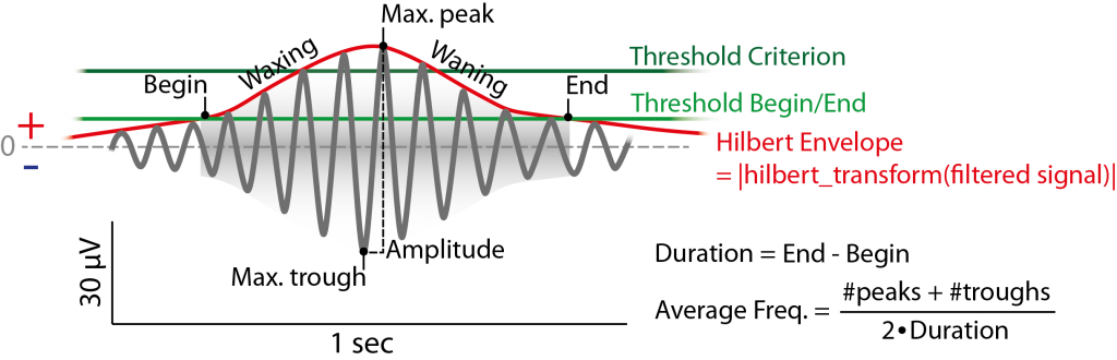
Figure 6.2: Example of (fast) spindle in the filtered signal (12-15 Hz) and its definition by the detection method used. Detection is based on two thresholds (green) passing the hilbert envelope of the filtered signal. Thresholds can be absolute Potential value, but usually are a multiples (e.g. 1.5 for the begin/end threshold, 2.25 for the criterion threshold) of the standard deviation (or the mean) of the whole filtered signal (e.g. of a respective channel) (or the envelope itslef).

 

Slow oscillation detection

Slow oscillation detection is based on (Mölle et al. 2002) but also see (Ngo et al. 2013). The algorithms were further adapted to get more properties and flexibility for finding slow oscillations as is described in the following. Prior to the actual detection, the signal is high pass filtered (IIR by default) then low pass filtered (FIR) to contain frequency components observed in slow oscillations in a specified band e.g. 0.3 to 3.5 Hz. This pre-filter assures that fast potential changes and components within a slow oscillation that are beyond the peak frequency are still considered even if the actual frequency of the slow oscillations is lower than required (e.g. 0.8 Hz). Then all the time intervals with consecutive positive-to-negative zero crossings are marked. Only intervals with durations corresponding to a minimum and maximum slow oscillation frequency are considered as putative slow oscillations. For example slow oscillations between 0.5 Hz and 1.25 Hz correspond to a time interval range of 0.8 to 2 s duration. These minimum and maximum frequencies are either given to be constant for all datasets or – like in spindle detection – can be given in dataset-specific center frequencies plus and minus a specific frequency bandwidth (however here further global limits like in spindle detection across datasets cannot be applied). For the putative slow oscillations the following properties are determined from the filtered signal:

• Duration/Length of a slow oscillation is the end minus the beginning time-point determined by the positive-to-negative zero (Down-zero-crossings). The samples that correspond to the “sample frequency per minimal slow oscillation frequency” are ignored at the borders of consecutive data blocks.
• The down-peak (or maximal trough) is the minimal potential in the filtered signal,if before a negative to positive zero crossing (Up-zero-crossing), and the up-peak (maximal peak) is the most positive potential following thereafter, and if before the end of the time interval. The up-peak and the down-peak potential are determined as the difference to zero in the filtered signal and are respective negative and positive potentials.
• The estimated slope is calculated by the down-peak potential (zero to down peak potential) over the time lag to the following Up-zero-crossing. Similarly a second slope estimate, the maximal slope, is calculated by the maximal difference in potentials between data-point samples in between down-peak and up-peak and the sample frequency giving the constant time lag between data-point samples. NEW: Also the slope from the first Down-zero-crossing to the down-state is now reported in addition.
• The amplitude (aka. maximum trough to peak potential) of the slow oscillation is the absolute difference in potential between up-peak and down-peak (up-peak potential minus down-peak potential).
• The average frequency of a slow oscillation is determined by the length of the slow oscillation, i.e. 1/ (length of slow oscillation). A second approximation is not by the length of the slow oscillatoin, but by the down-to-up-peak time lag.
• Samples and/or time-points of the begins, ends, down-peak, up-peak, slope, max slope, are also reported.
• Also the standard deviation within the filtered signal of the spindle is given to exclude further outliers after detection is finished.

Before further filtering putative slow oscillations can then be further excluded if they do not concur with a maximum up-peak or down-peak potential, given in absolute values of the potential (e.g. 800 µV).

Afterwards putative slow oscillations are further selected if their down-peak potential was lower than a factor (e.g. 1.25) times the mean down-peak potential and whose amplitude is larger than another factor (e.g. also 1.25) times the mean amplitude of all other putative detected slow oscillations within this channel. To also detect smaller slow oscillations the factors can be chosen smaller (e.g. 1.0 or 0.75 fo mean putative slow oscillation values). See Figure 7.

The final slow oscillations are ordered in time of occurrence, also given a specific identification index within each channel reflecting the temporal ordering.

Report of slow oscillations events includes each event and its properties (event file), and an aggregation by channels of interest with key mean or summary values (channel file). Files for each individual dataset are then merged to a single file containing all entries of all analyzed datasets.

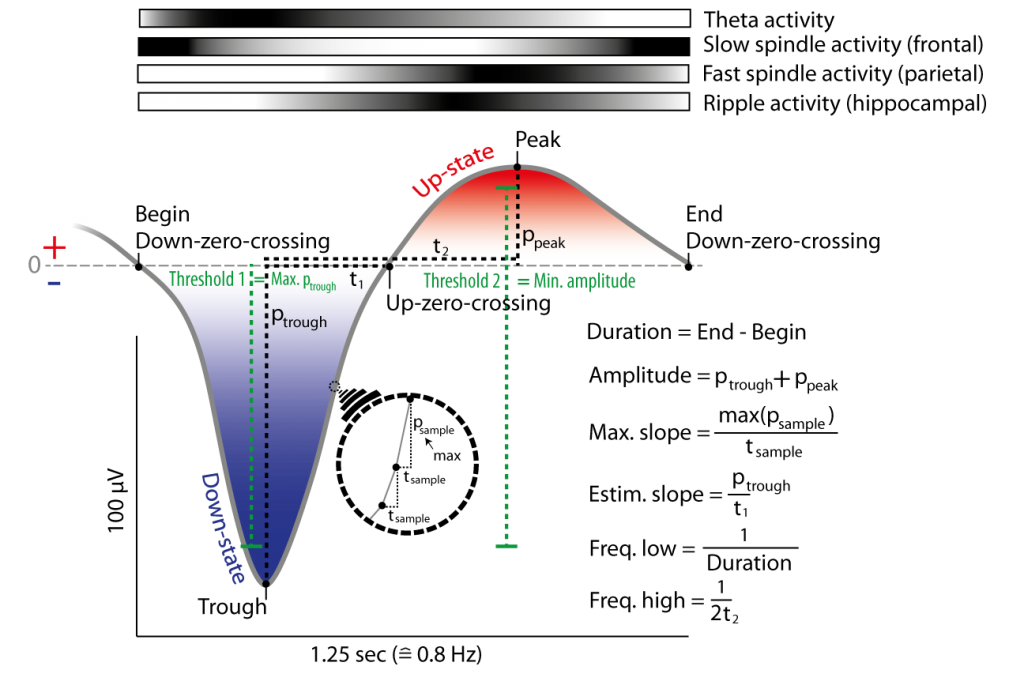
Figure 7: Example of a slow oscillation in the filtered signal (0.3 to 4 Hz) and its detection due to Down-zero-crossings (i.e. positive to negative potential change in filtered signal) and thresholds. Slow oscillations are defined between two Down-zero-crossings with delay matching slow oscillation frequencies (e.g. 0.5-1.25 Hz) and thresholds that mark the maximal negative down potential and the minimal necessary amplitude. Thresholds can be obtained by multiples (e.g. 1.25) of the mean over all candidates slow oscillations (of a channel) with Down-zero-crossings having delay matching slow oscillation frequencies. Slope and frequency of a slow oscillation is can be obtained by two methods each. The top of the figure depicts the probability of co-occurring events/activitry like fast and slow spindles on frontal and parietal cortex and hippocampal ripple activity (darker colors mean higher occurrence relative to lower (whiter) periods). Note there is less such activity during the down-state (as opposed to the preceding or following up-state) of the slow oscillation.

Non-events

Non-events are detected according to event time-points in respective matching sleep stages of interest. Matching is according to specified sleep stage resolution. For example NonREM has three further resolutions: (S2 + SWS) or (S2 + S3 + S4). If one gives SWS + S2 instead of NonREM, then an event in S2 is matched by a non-event in S2 and an event in SWS is matched by a non-event in SWS.

Given the time-points of events and a column that gives the respective channels of the events, they are further defined by a pre- and post-events time buffers, i.e. how long ago the event started previous to the given time-point (pre-event time buffer) and how long after the event it ends (post-event time buffer). For example if an event occurs at 203.5 s and the pre-event buffer is 1 s and the post event buffer is 1.5 s, then the event begins at 202.5 and ends at 205.0 s. Therefore these buffers define the left and right boundaries of the actual event and also the “to-be-found” non-events.

Further, two event-to-non-event-boundary time buffers are given, one to the left and one to the right. They further define the minimal distance difference of the boundaries (begins and ends) of new non-events to all the other events.

These four buffers and the to-be-matched sleep stage of interest are limiting the search space for non-events within a channel.

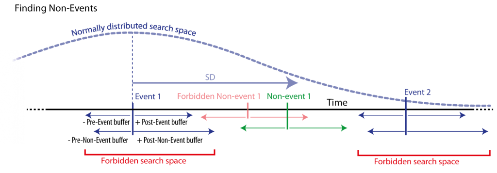
Figure 8: Non-event detection by searching for every event (blue) a corresponding non-event. Non-events are searched randomly in a time window with normally distributed distance from the corresponding event. Only non-events that match specified (buffered) distances form the event and other events are accepted. Those distances are defined by specific time buffers around events to non-events’ boundaries, i.e., a and minimal distance from events and non-events. Also, search spaces that are not of the same sleep stage can be forbidden (not shown here).

The search space can further be limited to consider events given in all other channels of interest.

Within those limits a non-event matching previous criteria is searched randomized following a normal distribution that is defined by a given standard deviation in seconds. A new non-event is not allowed to overlap with any already found non-events in the same channel. Note that two event boundaries of other events and all non-event-boundaries can also not overlap. If no matching non-event can be found in a given number of random tries, then the standard deviation is increased by a step size. Those increases are performed every such number of random tries until it reaches the given maximum of tries per event to find any non-event. In case of maximum number of tries (i.e. a rare case) the last guess of non-event is taken, that does not overlap with any event if it can take the time space of an already found non-event, therefore in this case the non-events can overlap. Note that this cannot be avoided if events are to densely packed for a sufficiently large search space for every event. In the case that non-events are too densely packed and do not allow for any non-event to be found in the search space (not considering other found non-events) until the maximum number of tires and any further try,  then non-events may overlap with events. To avoid sequence effects of filling the gaps in the allowed search space of possible non-events, the event time-points are processed in random order. However output is in the same order as the events given for input. Randomization is seeded, i.e. a seed (a positive natural number) is given, and allows the same random events and output given the same input when by using the same seed (changeing the seed changes the output though the input is the same). The output then contains an indexed,corresponding non-event for each given event.

 

Event co-occurrence

A list of test events (Tests or Seeds), i.e. time-points, are tested to fall within a list of further specified target events. Target events are time-points with an offset and a pre- and post- time window before this offset (Targets). Time windows can be defined by constant values or alternatively by two columns in the target dataset with two respective constant time offsets. See Figure 9.

Tests and Targets are listed in separate tables with their corresponding time-points and further columns on witch Test and Target can be further matched, i.e. if they should be compared. The columns used for comparison of Tests and Targets should match in content and number of columns. Test events are called Matches if they match a target and Mismatches if they do not.

Results are reported per Test, i.e. for each Test each matched Target is given in a line with the complete table content of the test and target events and further annotation. Note that one test can match several targets in some cases, and that this results in more than one entry of the same Test (or entry of the same Target). Results are split in separate files for Matches and Mismatches. Furthermore a summary file listing the matches and mismatches grouped by specified columns in the table of test events. Output is grouped in order of Test events in respective input table. Note that switching the Targets for the Tests can result in the same results, however differently grouped or ordered.  Also not that if Tests and Targets are from the same table this can be used to assess temporal overlap of events in a specific range (this would be the non-identical matches). Finally this can be used to compare two different results of detections (e.g. having used detections with different paramters).

Matches can be filtered for identical and duplicate matches, e.g. if matching the same events against themselves (for a delay/traveling analysis), then pairs of matches (Test-Target  or Target-Test will only occur once if already contained and Tests will move to the Mismatches if they would match twice in that matter. Same events this can also just be excluded to match itself according to identity markers (i.e. the combination of data columns to describe a unique event).

 

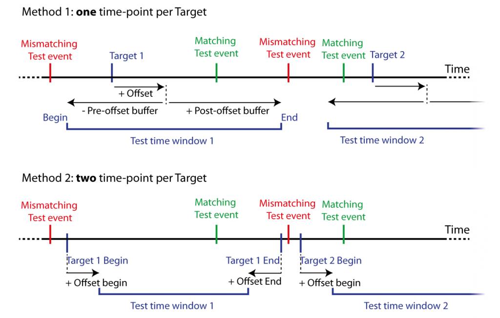
Figure 9: Two methods for matching event co-occurrence. Test events are matched against Target events defined by either one time-point and offset with pre- and post-offest time buffers (Method 1), or two time-points marking the begin and end of the target events with two respective offsets (Method 2). This defines time windows for Test events to fall within range of Target events, i.e., within a test time window. Matching Test events temporally fall (at least) within one of the test windows, mismatching Test events temporally fall within no test time window.

 

…A full Tutorial will be online sooner or later.

… for now I have given skype tutorials and workshops on how to use SpiSOP, you can contact spisop@spisop.org and ask for that, I am happy to help. Soon I will also publish a tutorial video, and give here good descriptions of the first steps, and a full tutorial, or how to deal with example data in detail, if you are unpatient, really just ask.

For now, find the quick-start guide for the standalone version and “experienced” useres already.

References

Heinzel, G., Rüdiger, A., Schilling, R., & Hannover, T. (2002). Spectrum and spectral density estimation by the Discrete Fourier transform (DFT), including a comprehensive list of window functions and some new flat-top windows. Max Plank Institute, 12, 122.

Mölle, M., Marshall, L., Gais, S., & Born, J. (2002). Grouping of spindle activity during slow oscillations in human non-rapid eye movement sleep. The Journal of neuroscience, 22(24), 10941-10947.

Ngo, H. V., Martinetz, T., Born, J., & Mölle, M. (2013). Auditory closed-loop stimulation of the sleep slow oscillation enhances memory. Neuron, 78(3), 545.

Rechtschaffen, A., & Kales, A. (1968). A manual of standardized terminology, techniques and scoring system for sleep stages of human subjects.